- In Linux, all processes and threads get a unique identifier (ID) and are all listed as directories of the same level under the
/procpseudo file system. - These processes and threads are represented as subdirectories in the form of
/proc/[pid], where thepidis the unique numerical ID for each. - So, technically, the “
pid” is not just a process ID but could be an ID for either a thread or a process. htopshows both processes and threads, and doesn’t distinguish them by default.- Consequently, its “PID” column contains IDs for both processes and threads.
- This dreadful terminology overloading has a historical reason:
- Linux originally didn’t have the notion of threads.
- It only had separate processes, each of which has a unique
pid, potentially sharing some resources like virtual memory and file descriptors. -
In 2001, Linux 2.4 introduced “Thread groups”, which gave rise to threads within a process. From the clone(2) man page:
Thread groups were a feature added in Linux 2.4 to support the POSIX threads notion of a set of threads that share a single PID. Internally, this shared PID is the so-called thread group identifier (TGID) for the thread group. Since Linux 2.4, calls to
getpid(2)return the TGID of the caller.- So, the PID of the parent process is overloaded with another meaning, the TGID :)
- That’s said, the kernel still doesn’t have a separate implementation for processes and threads.
- In summary, threads within a process will get the same PID , while each of which has a unique thread ID (TID).
- The values returned by the
getpid()are the same for all of them. - But the TID from the
gettid()are always unique.
- The values returned by the
How to Distinguish between a Thread and a real “Process”?
- As mentioned above, threads and process are similar in nature (kernel implementation), and both are “schedulable” entities to the kernel.
- The main difference between them is the scope of their namespaces (address space, resources, etc.).
- To distinguish between threads and processes, we need to look into the
/proc/[pid]/task/[tid]subdirectories wheretidis the kernel thread ID. - Kernel threads are the ones registered in and scheduled by the kernel.
- There are user-level threads (e.g., Java threads) invisible to the kernel and managed by the application layer.
- See here for more.
- The threads within parent process are under the same thread group (TG) umbrella, having the same TGID as the main thread but different
tids.- The main thread is the “process” that spawned all the children threads and has the same TGID as its PID.
/proc/[pid]/task/[tid]shares the same content as/proc/[pid]/ifpid==tid, i.e., it contains the same information describing the same process/thread.- Therefore, when you look into the
/proc/[pid]directory of a multithreaded process:- The
task/[tid]subdirectories are all the threads within the same thread group. - They have the same TGID being the
pid. - The so-called process is the main thread that spawned all other threads.
- The main thread has the same TGID as its PID (usually the smallest one under the
task/directory).
- The
Last Note: Multiprocessing vs. Multithreading
- To avoid confusion, apart from the thread group ID (TGID), there is also a process group ID (PGID).
- The former is for multithreading, and the later is used in multiprocessing.
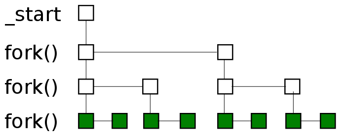
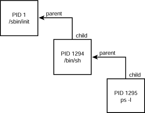
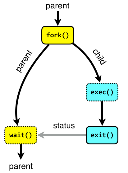
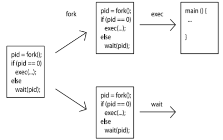
- A process is spawned by invoking the
fork()syscall, a thread is created by e.g.,pthread_create()in C. (Under the hood, they all use the syscallclone()but with different parameters)- The process that spawns other subprocesses is the parent.
- When spawning a new process, the parent can either create a new process group (and puts itself and its children into it) or inherits that of an existing process (usually it’s the grandparent process).
- If a new process group is created, the PGID will be the PID of the process that creates it.
- If it’s inherited, the PGID is the same as that of the grandparent.
- The process (the main thread) and all the threads it creates are siblings.
- They share the same TGID.
- They also have the same PGID as that of the main thread.
- NB: The threads created by a process are NOT visible to its parent process.
- The process that spawns other subprocesses is the parent.
Example
- We easily can launch a multithreaded program with
stress-ngon Linux. - A “stressor/hog” is a process.
-
We can run the stress test for memory accesses with the following command, which will spawn a stressor that runs with 5 threads reading and writing to two different mappings of the same underlying physical page.
hy@node-0:~$ stress-ng --mcontend 1 -t 10h stress-ng: info: [56472] dispatching hogs: 1 mcontend -
With
htop, we can see the process and threads therein in hierarchy (thePGRPis the GPID, and thePIDis the ID for threads/processes).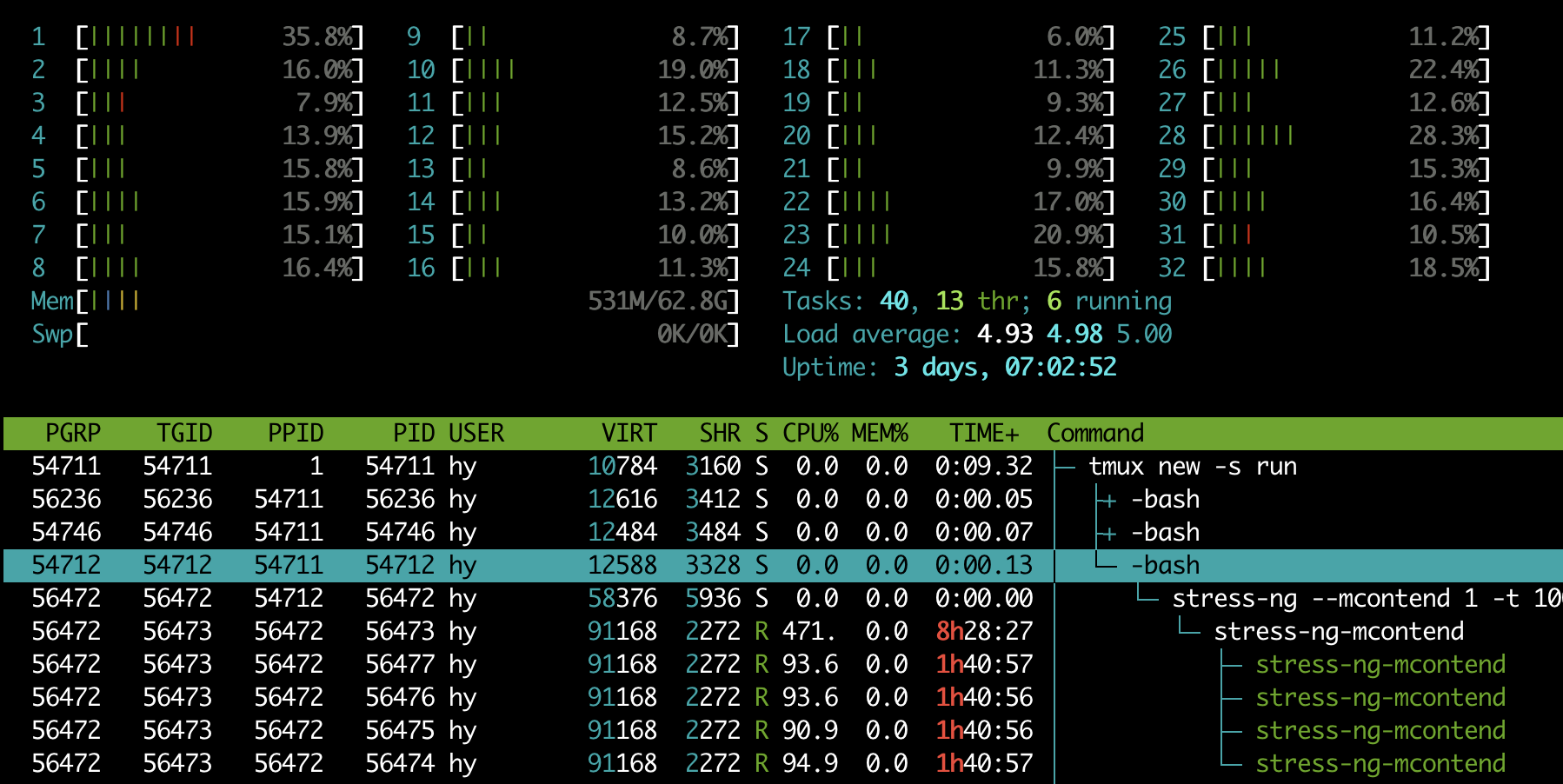
- We can see that all the threads and processes have a unique ID,
PID(process/thread ID).56472: The single-threaded parent process spawned from the bash command.56473: The multithreaded child process (and the main thread) spawned from the parent56472.56473-56477: The 5 sibling threads created by the main thread56473.
- We can see that all the threads and processes have a unique ID,
-
Then, by using
pidof, we get thepidof the main thread.hy@node-0:~$ pidof stress-ng-mcontend 56473 -
Since the bash command
56472is the parent process that spawned the child process56473, we can examine this relationship by checking:hy@node-0:~$ cat /proc/56472/task/56472/children 56473 -
Then, navigate to the
/procdirectory and check the/proc/[pid]/task/subdirectories. We get the 5 threads within this process:hy@node-0:~$ ll /proc/56473/task/ total 0 dr-xr-xr-x 7 hy hy 0 Dec 31 22:21 ./ dr-xr-xr-x 9 hy hy 0 Dec 31 22:21 ../ dr-xr-xr-x 7 hy hy 0 Dec 31 22:21 56473/ dr-xr-xr-x 7 hy hy 0 Dec 31 22:21 56474/ dr-xr-xr-x 7 hy hy 0 Dec 31 22:21 56475/ dr-xr-xr-x 7 hy hy 0 Dec 31 22:21 56476/ dr-xr-xr-x 7 hy hy 0 Dec 31 22:21 56477/ -
To examine directory of a child thread, we get the same output as above since they are siblings.
hy@node-0:~$ ll /proc/56476/task/ total 0 dr-xr-xr-x 7 hy hy 0 Dec 31 22:21 ./ dr-xr-xr-x 9 hy hy 0 Dec 31 22:21 ../ dr-xr-xr-x 7 hy hy 0 Dec 31 22:21 56473/ dr-xr-xr-x 7 hy hy 0 Dec 31 22:21 56474/ dr-xr-xr-x 7 hy hy 0 Dec 31 22:21 56475/ dr-xr-xr-x 7 hy hy 0 Dec 31 22:21 56476/ dr-xr-xr-x 7 hy hy 0 Dec 31 22:21 56477/ -
Note that the parent process
56472is a single-threaded process, so its/taskdirectory contains only itself.hy@node-0:~$ ll /proc/56472/task/ total 0 dr-xr-xr-x 7 hy hy 0 Dec 31 22:21 ./ dr-xr-xr-x 9 hy hy 0 Dec 31 22:21 ../ dr-xr-xr-x 7 hy hy 0 Dec 31 22:21 56472/
Resource Accounting
- The resource usage of a process/thread can be obtained in various ways, and the information is not consistent.
- From above,
htopaggregate all the resource usages in the main thread56473by default. - We can obtain per-process information from
psas well:-
Like
htop, It aggregates usage of all threads to the main threads by default.hy@node-0:~$ ps -p 56473 -o %cpu,%mem,cmd %CPU %MEM CMD 473 0.0 stress-ng-mcontend -
It only works on the main thread but not with the siblings:
hy@node-0:~$ ps -p 56476 -o %cpu,%mem,cmd %CPU %MEM CMD -
To see detailed thread-level information, we can use the
-Lflag on the main thread:hy@node-0:~$ ps -L 56473 -o %cpu,%mem,cmd %CPU %MEM CMD 97.3 0.0 stress-ng-mcontend 94.0 0.0 stress-ng-mcontend 94.0 0.0 stress-ng-mcontend 94.0 0.0 stress-ng-mcontend 94.0 0.0 stress-ng-mcontend -
With
-Foption, we can obtain the full glory:hy@node-0:~$ ps -L 56473 -F UID PID PPID LWP C NLWP SZ RSS PSR STIME TTY STAT TIME CMD hy 56473 56472 56473 97 5 22792 2604 13 08:10 pts/2 RLl+ 302:30 stress-ng-mcontend hy 56473 56472 56474 94 5 22792 2604 7 08:10 pts/2 RLl+ 292:03 stress-ng-mcontend hy 56473 56472 56475 94 5 22792 2604 31 08:10 pts/2 RLl+ 292:00 stress-ng-mcontend hy 56473 56472 56476 94 5 22792 2604 15 08:10 pts/2 RLl+ 291:59 stress-ng-mcontend hy 56473 56472 56477 94 5 22792 2604 0 08:10 pts/2 RLl+ 292:05 stress-ng-mcontend -
Note that ALL threads share the same PID but each of them has a unique TID (
LWP).
-
-
We can monitor those threads using
topwith-H:hy@node-0:/proc$ top -H -p 56476 .... PID USER PR NI VIRT RES SHR S %CPU %MEM TIME+ COMMAND 56473 hy 20 0 91168 2708 2272 R 97.3 0.0 127:24.91 stress-ng-mcont 56474 hy 20 0 91168 2708 2272 R 94.0 0.0 122:55.16 stress-ng-mcont 56475 hy 20 0 91168 2708 2272 R 94.0 0.0 122:54.44 stress-ng-mcont 56476 hy 20 0 91168 2708 2272 R 93.7 0.0 122:55.33 stress-ng-mcont 56477 hy 20 0 91168 2708 2272 R 92.3 0.0 122:56.57 stress-ng-mcont-
Without the
-Hflag, however, it aggregates all usages to any of the sibling threads:hy@node-0:~$ top -p 56476 .... PID USER PR NI VIRT RES SHR S %CPU %MEM TIME+ COMMAND 56473 hy 20 0 91168 2708 2272 R 476.3 0.0 621:39.36 stress-ng-mcont -
Also, we can get a single number out:
  # Get the CPU utilization of thread 56476.
  # * Aggregated.
  hy@node-0:~$ top -b -n 2 -d 0.2 -p 56476 | tail -1 | awk '{print $9}'
  465.0
  # * Per-thread with -H.
  hy@node-0:~$ top -b -H -n 2 -d 0.2 -p 56476 | tail -1 | awk '{print $9}'
  75.0
-
- How to get per-thread resource usages? We need to again look into the
/procsysfs.- The file
/proc/pid/statof a thread (whose TID==pid) contains the information aggregated from all threads. -
The file
/proc/pid/task/pid/statcontains per-thread information:# * Get total cpu time (user and kernel) of all threads belonging to the same TG as that of 56476. hy@node-0:~$ cat /proc/56476/stat | awk '{print $14, $15}' 9460932 12361 # * Get the cpu time for only thread 56476. hy@node-0:~$ cat /proc/56476/task/56476/stat | awk '{print $14, $15}' 1879429 3032
- The file
-
Alternatively, we can use the mighty python with
psutil.>>> import psutil # The great grandparent process. >>> tmux_session = psutil.Process(54711) # * It's spawned from the mother of all processes of PID=1 -- the init(old distros)/systemd(new distros). >>> tmux_session.ppid() 1 >>> [(child.name(), child.pid) for child in tmux_session.children(recursive=True)] [('bash', 54712), ('bash', 56236), ('python', 56613), ('stress-ng', 56472), ('stress-ng-mcontend', 56473)] # The parent process. >>> parent = psutil.Process(56472) # * The parent was spawned from one of the above bash sessions (grandparent) >>> parent.ppid() 54712 # * The sibling threads art NOT children, and invisable to the parent process. >>> parent.children(recursive=True) [psutil.Process(pid=56473, name='stress-ng-mcontend', status='running', started='11:21:57')] # * The parent is single-threaded. >>> parent.num_threads() 1 # The child process spawned from the parent process. >>> child = psutil.Process(56473) # * The child created 5 threads (including itself). >>> child.num_threads() 5 >>> [thread.id for thread in child.threads()] [56473, 56474, 56475, 56476, 56477] # One of the sibling threads. >>> sibling = psutil.Process(56476) # * The sibling thread inherits the parent process of the main thread. >>> child.ppid() 56472 >>> sibling.ppid() 56472 # Accounting resouces. # * The parent process is in sleep state (S), so it doesn't take any CPU time. >>> parent.cpu_percent(interval=1) 0.0 # ! psutil **aggregates** all sibling resources to **any** of the siblings. >>> sibling.cpu_percent(interval=1) 471.5 >>> child.cpu_percent(interval=1) 472.4 # ! Also, its cpu time accounting for children processes is broken somehow ... >>> tmux_session.cpu_times() pcputimes(user=7.46, system=3.19, children_user=102.18, children_system=153.15, iowait=0.0) >>> parent.cpu_times() pcputimes(user=0.0, system=0.0, children_user=0.0, children_system=0.0, iowait=0.0) >>> child.cpu_times() pcputimes(user=45250.11, system=57.79, children_user=0.0, children_system=0.0, iowait=0.0) >>> sibling.cpu_times() pcputimes(user=45255.42, system=57.79, children_user=0.0, children_system=0.0, iowait=0.0) # * Memory usages are accounted the same as it does for CPU. >>> parent.memory_full_info() pfullmem(rss=6475776, vms=59777024, shared=6078464, text=1728512, lib=0, data=32018432, dirty=0, uss=3051520, pss=3749888, swap=0) >>> child.memory_full_info() pfullmem(rss=2772992, vms=93356032, shared=2326528, text=1728512, lib=0, data=65581056, dirty=0, uss=126976, pss=735232, swap=0) >>> sibling.memory_full_info() pfullmem(rss=2772992, vms=93356032, shared=2326528, text=1728512, lib=0, data=65581056, dirty=0, uss=126976, pss=735232, swap=0) >>> tmux_session.memory_percent() 0.007239506814671662 >>> parent.memory_percent() 0.009602063988251591 >>> child.memory_percent() 0.004111699759675096 >>> sibling.memory_percent() 0.004111699759675096 - In summary, there are various ways of accounting resources for processes and threads on Linux.
- However, there are nuances that must be taken into account.
psutilis a convenient tool for sys admins when scripting in python.- However, the resource usage of any threads is the aggregated values of all threads!
- It doesn’t explicitly distinguish between PIDs and TIDs either.
-
And it’s time to end our running example:
  # ! "Note this will return True also if the process is a zombie (p.status() == psutil.STATUS_ZOMBIE)"
  >>> parent.is_running() == child.is_running() == sibling.is_running() == True
  True

  >>> import signal
  >>> sibling.send_signal(signal.SIGINT)

  >>> parent.is_running() == child.is_running() == sibling.is_running() == False
  True
(It seems that interrupting one thread has a bottom-up cascading effect in
stress-ng🥴 )
Happy New Year 🎆 ~
Reference
- https://unix.stackexchange.com/questions/364660/are-threads-implemented-as-processes-on-linux
- https://unix.stackexchange.com/questions/670836/why-do-threads-have-their-own-pid
- https://stackoverflow.com/questions/1221555/retrieve-cpu-usage-and-memory-usage-of-a-single-process-on-linux
- https://unix.stackexchange.com/questions/404054/how-is-a-process-group-id-set
- https://stackoverflow.com/questions/4856255/the-difference-between-fork-vfork-exec-and-clone
- https://stackoverflow.com/questions/19678954/relation-between-thread-id-and-process-id
- https://stackoverflow.com/questions/9430491/find-cpu-usage-for-a-thread-in-linux
- https://stackoverflow.com/questions/1420426/how-to-calculate-the-cpu-usage-of-a-process-by-pid-in-linux-from-c
- https://stackoverflow.com/questions/19919881/sysconf-sc-clk-tck-what-does-it-return
- https://www.baeldung.com/linux/total-process-cpu-usage
- https://psutil.readthedocs.io/en/latest/#processes
- https://man7.org/linux/man-pages/man5/proc.5.html
- https://man7.org/linux/man-pages/man2/getpid.2.html
- https://man7.org/linux/man-pages/man2/gettid.2.html
- https://manpages.ubuntu.com/manpages/bionic/man1/stress-ng.1.html
- https://www.akkadia.org/drepper/nptl-design.pdf