Single-Source Shortest-Paths (Dijkstra Algorithm)

⚠️ This post was created when I was in high school and is no longer maintained.

1. Recall the basics

• Unlike the Bellman-Ford algorithm where the edge weights can be negative, Dijkstra’s algorithm solves the single-source shortest-paths problem on a weighted, directed graph $G = (V, E)$ for the case in which all edge weights are nonnegative.

• The Bellman-Ford algorithm relaxes each edge $V - 1$ times, whilst Dijkstra’s algorithm ( as well as the shortest-paths algorithm for directed acyclic graphs ) relax each edge exactly once.

• With a good implementation, the running time of Dijkstra’s algorithm is generally lower than the Bellan-Ford algorithm.

• It is akin to the breadth-first search in that set $S$ corresponds to the set of black vertices in a breadth-first search; just as vertices in $S$ have their final shortest-path weights, so do black vertices in a breadth-first search have their correct breadth-first distances.

• It is like Prim’s algorithm as both algorithms use a minpriority queue to find the “lightest” vertex outside a given set.

• The loop invariant that Dijkstra’s algorithm maintains is $Q = V - S$

• As mentioned above, Dijkstra’s algorithm always chooses the “lightest” or “closest” vertex in ${V - S}$ to add to set $S$, we say that it uses a greedy strategy.

• Greedy strategies do not always yield optimal results in general, but as the following theorem and its corollary show, Dijkstra’s algorithm does indeed compute shortest paths.

---

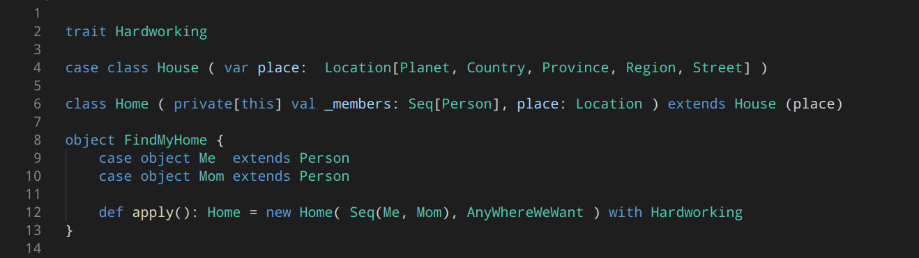
2. Pseudocode

-- the same preparation as before --
struct SSNode {
    double d;
    SSNode* π;
};
algorithm InitialLizeSingleSource(G, sourceNode):
    For node in G do
        node.d := +INF
        node.π := NIL
        
    sourceNode.d := 0

{- `Relaxation()` is nothing but examining whether or not
 - by using the new "pit stop" (`u`) can reduce the price
 - (`d`) of the node `v`.
 -}

algorithm Relax(u, v, (*CalcWeight)(_, _)):
    if v.d > u.d + CalcWeight(u, v) then
        v.d := u.d + CalcWeight(u, v)
        v.π := u


algorithm Dijkstra(G, (*CalcWeight)(_, _), sourceNode):
    InitialSingleSource(G, sourceNode)
    
    DeterminedNodes := Ø
    Q := new MinQueue(G.V, key=node.d)
    
    While Q != Ø do
        u := ExtractMin(Q)
        DeterminedNodes += u
        -- obtain u's outgoing edges from u's adjacency list and relax them all --
        For node in G.adj[u] do 
            Relax(u, node, CalcWeight)

---

3. Time Complexity

The running time of Dijkstra’s algorithm depends on how we implement the min-priority queue.

• The outer while-loop has exactly $ \mid V \mid $ interations in which 2 Min-Queue operations, ExtractMin() and Insert(), are carried on;

• The inner for-loop, where DecreaseKey() get called implicitly, iterates $ \mid E \mid $ times, since the total number of edges in all the adjacency lists is $ \mid E \mid $;

1) Use array: we maintain the min-priority queue by taking advantage of the vertices being numbered 1 to $ \mid V \mid $ and we simply store $v.d$ in the vth entry of an array. (similar to the direct-address hashing )

• Insert() and DecreaseKey(): $O(1)$ time
• ExtractMin(): $O(V)$ time (since we have to search through the entire array))

\[O( \mid V \mid ^2 + \mid E \mid ) \in O( \mid V \mid ^2)\]

2) Use binary minheap: For the case where the graph is sufficiently sparse. ( the implementation should make sure that vertices and corresponding heap elements maintain handles to each other. )

• ExtracMin() and DecreaseKey(): $O(lg V)$ time
• BuildMinHeap(): $O(V)$ time

\[O( \mid V \mid + \mid E \mid ) \cdot lg \mid V \mid ) \in O( \mid E \mid lg \mid V \mid )\]

3) Use Fibonacci heap: (see CRLS Chapter 19)